Exploring Parallel Computer Architecture with FPGAs
RISC-V Composable Extensions for MX Microscaling Data Formats for AI Tensors: Part One: Introduction to MX Data
In this post we review the design and history of MX format reduced precision block floating point vector data formats. In the next post, we explore several possible RISC-V composable custom extensions to compute over them.
Microsoft team demonstrates a more frugal way to do AI tensor math, rivals unite in support
This MX Alliance proposes standards for new 4b, 6b, 8b floating point element and 8b integer element block floating point formats that are poised to obsolete use of 16-bit and wider floating point formats within matrix multiplies and convolutions in machine learning training and inference workloads.
A block floating point format replaces the k exponent terms of the individual elements of a block of k elements with a single common scaling term, X, stored once. All elements’ mantissas are scaled for that X term. This significantly reduces the block’s memory footprint, and dramatically reduces the logic resources (ASIC gates or FPGA LUTs) required to implement vector operators (esp. vector dot product). The Spec:
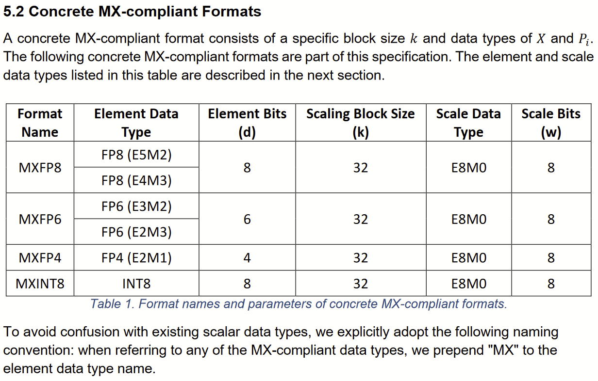
For MX formats, blocks have k=32 elements, the scale factor X is an 8b exponent, and elements may be FP4, FP6, FP8, or INT8:
Thus a 32 element MXFP6 block requires 32×6b element data + 8b scale data = 200 bits, and a 256 element vector, in memory, might use 8 MXFP6s = 200 bytes (or more!).
The accompanying whitepaper Microscaling Data Formats for Deep Learning, evaluating various MX formats on real ML workloads, justifies the interest and expected uptake of these formats. For example, the paper finds “MXFP6 closely matches FP32 for inference after quantization-aware fine tuning” and “generative language models can be trained with MXFP4 weights and MXFP6 activations and gradients incurring only a minor penalty in the model loss.”
For these AI tensor math workloads, MX format data achieves comparable accuracy using only a small fraction of the circuit resources of FP32 data.
A curiously unspecific specification
The spec declines to specify such essentials as: 1) a canonical in-memory representation of MX data; 2) the required internal precision and final precision of MX dot product; and 3) besides element-wise conversion to/from float32, and dot product, what other MX operations are required, and at what internal and final precision? For example:
5.1 Microscaling (MX): “The layout of the block in physical memory is not prescribed in this specification.”
6.1 Dot Product of Two MX-compliant Format Vectors: “The dot product of two MX-compliant format vectors of length k is a scalar number C. … The internal precision of the dot product and order of operations is implementation defined.”
Also, per 6.2 General Dot Product, the dot product of two arbitrary vectors is the sum of the dot products of their constituent MX k-vectors, with type float32. Here again the specification does not prescribe the type, precision, or order of evaluation of the intermediate sums terms (if any).
Leaving these details unspecified is problematic. Diverse “compliant” MX libraries and cores will evaluate the same models but with different results. Perhaps these omissions are intentional, and necessary to secure endorsements from rivals with quite different means of evaluating MX dot products.
George Constantinides (Imperial College) also writes about this here: Industry Coheres around MX? “To my mind, the problem with this definition is that × (on elements), the (elided) product on scalings and the sum on element products is undefined. …”
Paper trail
Now let’s review prior work that (I believe) led these researchers to these new data formats.
Project Catapult at ISCA 2014
Project Catapult. Putnam et al, A Reconfigurable Fabric for Accelerating Large-Scale Datacenter Services, ISCA 2014. DOI. PR. This well cited paper documents Microsoft’s early Project Catapult work to use parallel FPGA overlay architectures, across myriad FPGAs, to accelerate Bing query document ranking at scale. “We describe a medium-scale deployment of this fabric on a bed of 1,632 servers, and measure its efficacy in accelerating the Bing web search engine.” (I built the §4.6. Document Scoring gadget stage of this ranking pipeline; working with the MSR and Bing teams was a career highlight.) I believe Catapult spurred Intel to acquire Altera for $17B in 2015.
Project Catapult’s investments in people and in datacenter-networked FPGAs hosting hardware microservices planted the seeds of Project Brainwave.
Project Brainwave at Hot Chips 2017
Project Brainwave. Chung and Fowers, Accelerating Persistent Neural Networks at Datacenter Scale, Hot Chips 2017. Video. The public debut of Brainwave. Leveraging FPGA hardware microservices at massive scale, it achieves high throughput, peak hardware utilization, and very low latency for batch size = 1 workloads, by keeping then-enormous ML models, many millions of parameters, entirely in SRAM across thousands of FPGAs’ × thousands of BRAMs, using tens of TBs/s/FPGA of SRAM bandwidth.
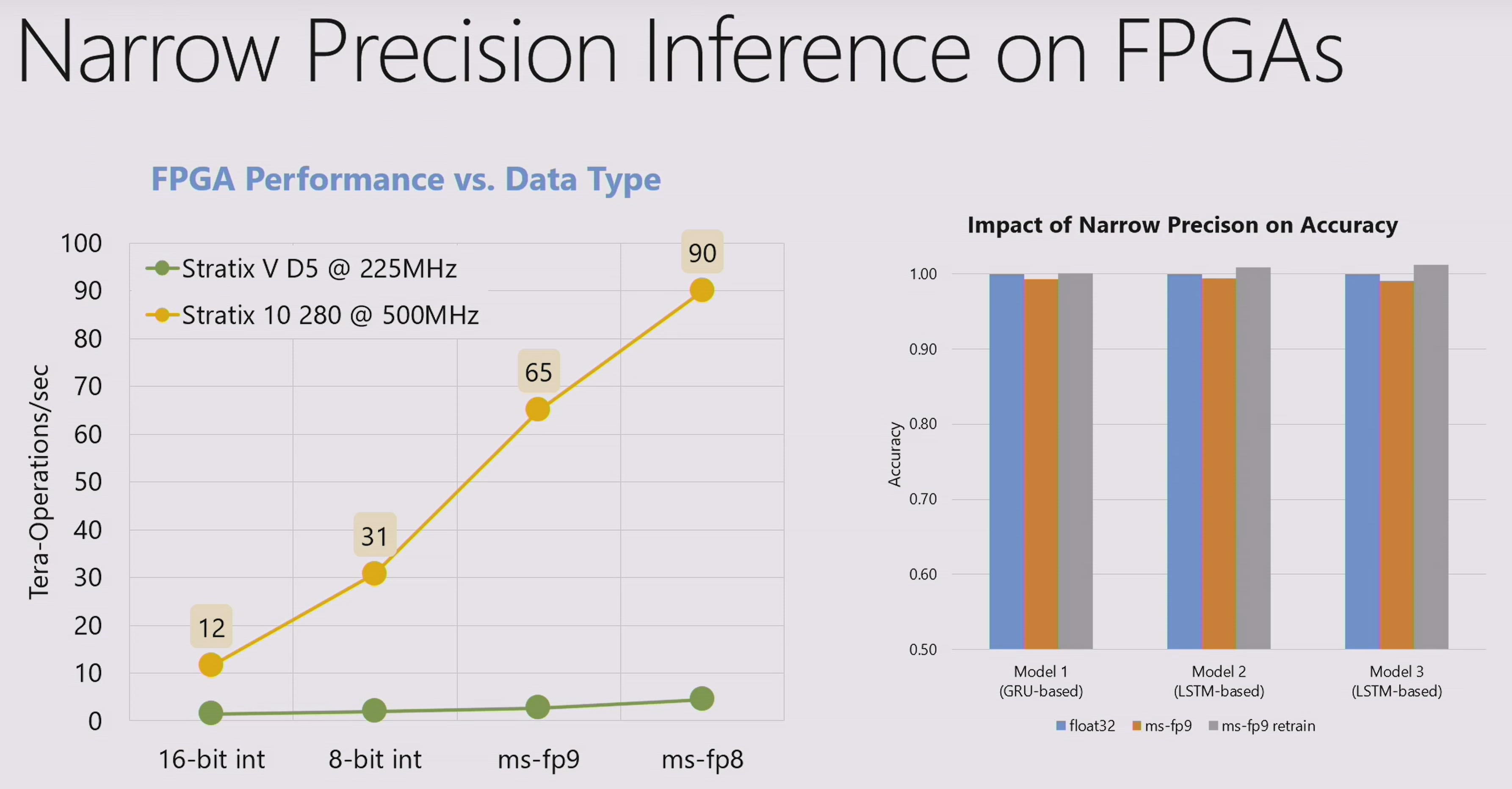
Fowers detailed the Brainwave soft DPU microarchitecture, including thousands of dot product units, totaling ~96,000 FMACs using narrow precision MS-FP floating point format: 90 TOPS ms-fp8 at 720 GFLOPS/W on Stratix 10 280. Despite quantization, its inference accuracy was comparable to float32 (after some retraining).
Brainwave’s mysteriously good floating point throughput
At the time I wondered, “How did Microsoft hit 90 TOPS? The no. of Stratix 10 DSPs × DSP Fmax << 90 TOPS. So some/most Brainwave FPUs must be in soft logic (LUTs). But 90 TOPS?! How?” To reproduce their result, I carefully designed frugal 8b and 6b FPUs, for Virtex UltraScale+ FPGAs. Try as I might, I couldn’t get to 90 TOPS. I wrote in 2017:
#FPGA noodling on LUT-frugal reduced precision floating point. fp8 = fp8*fp8 fp8 = fp8+fp8 fix16 += fp8*fp8 // commutative sum Thinking { sign:1; exp:4; mant:3 } per Deep CNN Inference with Floating-point Weights and Fixed-point Activations, flush-to-zero. For fp8 ::= { s:1; e:4; m:3 }, fp11 ::= { s:1; e:4; m:6 }: fix16 += (fp8)(fp8*fp8); // ~38 LUTs fix16 += (fp11)(fp8*fp8); // ~46 LUTs Pipelined at 500 MHz, in 1.2 M LUT XCVU9P * 90% utilization => ~28000 instances of fix16 += (fp8)(fp8*fp8) => 28 TFLOPs. (20+ TFLOPS in F1?) Eats 2*28K=56 KB/cycle. In a VU9P: 2160 BRAMs * 8 B/BRAM = 17KB/cycle; 960 URAMs * 16 B/URAM = 15KB/cycle. So requires weight or activation reuse. (Compare with XNOR-Net: 36b dot product = 50 LUTs per FPGA Hacks: Population count; VU9P URAM+BRAM bandwidth: 294Kb/cycle => ~300 TOPS @500 MHz with operand reuse.) For fp6 ::= { s:1; e:3; m:2 }, fp8x ::= { s:1, e:3; m:4 }: fix10 += (fp6)(fp6*fp6); // ~21 LUTs fix10 += (fp8x)(fp6*fp6); // ~24 LUTs Pipelined at 500 MHz, in 1.2 M LUT VU9P * 90% util => ~51000 instances of fix10 += (fp6)(fp6*fp6) => 51 TFLOPs. (40 TFLOPS on F1?) Even fp6 doesn’t match Brainwave’s “90 TFLOPs ms-fp8” on 500 MHz Stratix-10. Perhaps they are not using fused fp-mul-accumulate?
Multiplying is easy, young man, adding is harder
Where do the LUTs go in reduced precision FPGA FMACs?
First let’s adopt the MX Spec notation: “ExMy: Notation for a scalar format with one sign bit, x exponent bits, and y mantissa bits. E.g., E4M3 refers to an FP8 format with one sign bit, four exponent bits, and three mantissa bits.” (Mantissa bits is a misnomer here; these are fraction bits (after the binary point), not including the implicit leading 1., or 0. when the number is a denormal.) So working in E4M3 { s:1; e:4; f:3; }, that’s a 1b sign, 4b exponent, and 3b fraction(i.e., a 4b significand with an implied leading 1). It exactly represents certain real numbers such as 240.0 (+1.1112 x 27) and -1.02 x 2-7 = -.0078125.
It is inexpensive to multiply such low precision floats in 6-LUT FPGAs. For example assume (flush-to-zero) normalized E4M3 × E4M3 products have a target precision of E4M6. The product of two E4M3 1.f 4b significands lie in [1.0000002 , 11.1000012]. If the product >= 2.0, normalize it by shifting the binary point to the left, i.e., 1.11000012 x 2-1, and round/truncate the (underlined) least significant bit. Then multiplication is just a table lookup of the resulting 6b fraction after normalization and rounding. With 3b fraction inputs a.f and b.f you require 23+3 = 64 entries, perfect for a 6 6-LUT 64x6b ROM. Add one LUT for the (>=2.0) shift signal and 0.5 of a 5,5-LUT for the XOR of the sign bit. Add 0.5-2 LUTs for zeroes. The (twice biased) product exponent is (a.e + b.e + shift), 4 LUTs. In all, perhaps 14 LUTs and two LUT delays. Cheap.
The greater cost of the dot product’s multiply-accumulate is the adder / adder tree. The sum of (e.g.) four element-wise products 1×2-6 + 1×2-4 + 1×2-2 + 1×20 = 1.0101012 x 20. Naively each add requires a pre-addition shifter to align mantissas, an add/sub, and then a CLZ circuit and another shifter to renormalize the sum/difference. How wide those shifters are, how wide the sum reduction adder precision is, ideally, depends on the adder tree requirements. But compared to the two LUT delays of of the multiplier, this FP reduction adds more LUT delays / pipeline stages as well as area. “It all adds up.”
My 2017 preference was and is to keep the vector reduction sum in fixed point and first convert each product mantissa term to fixed point with a barrel shifter, the shift count controlled by the product term’s exponent. Then reduction order doesn’t matter — fixed point adds are commutative. When I tried this in 2017:
So the above ~14 LUT multiply incurs an additional ~16 LUT shift and ~16 LUT add/sub. Roughly 2/3 of the FMAC is the adder. Ouch. How does that translate into TOPS? For an XCVU9P device, 1.2 MLUTs × 0.9 / 38 LUTs/mulacc = ~28000 mulaccs × 2 ops/clock × 0.5 GHz = 28 TOPS.
I tried again with 6b×6b floating point but that only reached ~50 TOPS.
About half of Microsoft’s 90 TOPS result, in a comparable one million 6-LUT device. I was stumped.
Then came: Chung et al, Serving DNNs in Real Time at Datacenter Scale with Project Brainwave, IEEE Micro, March 2018. DOI. The Hot Chips follow-on IEEE Micro paper made things somewhat clearer: the 90 TOPS result is for msfp8 format, with a 2b fraction, at 550 MHz. More like my fp6 than my fp8. But the 90 TOPS result was still out of reach!
Brainwave at ISCA 2018, MSFP revealed as block floating point
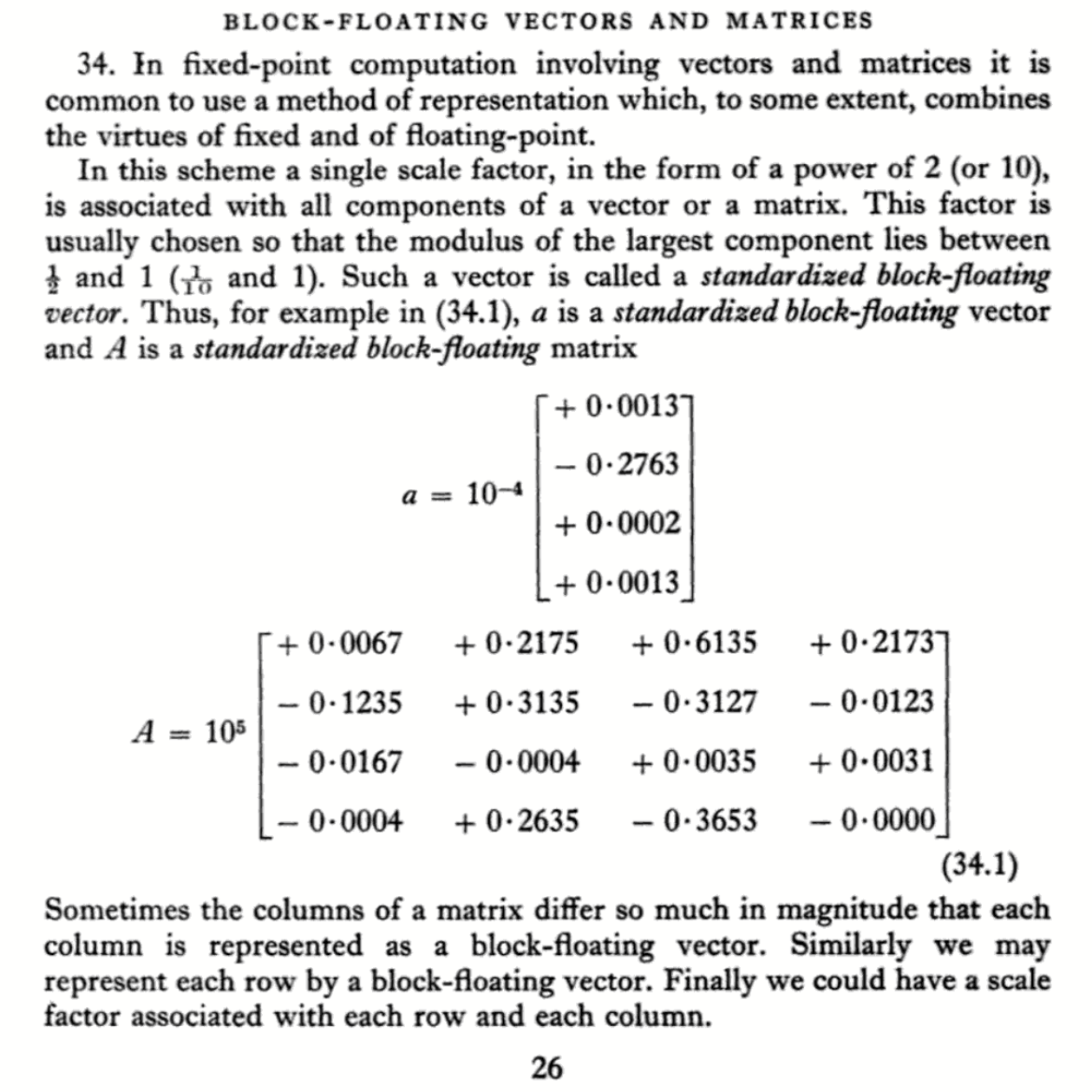
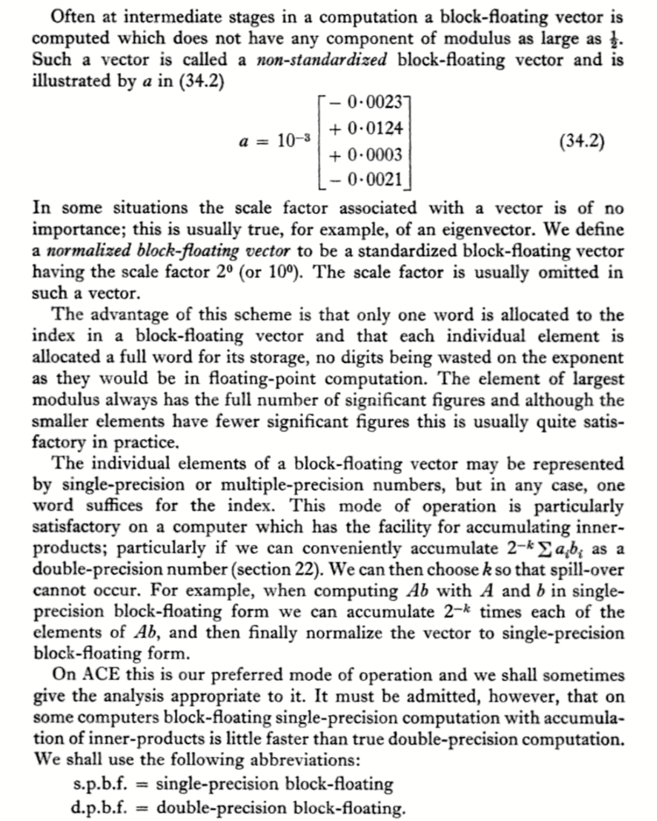
This paper details the Brainwave cloud scale DNN system, top to bottom, including the design of the Brainwave Neural Processor Architecture (NPU) SoC. It reveals the representation trick behind the highly efficient MS-FP datatypes — block floating point formats, recoding vector elements to use a common scaling factor, instead of per-element exponent scaling. This dates back at least to J.H. Wilkinson, “Block-floating vectors and matrices”, pp. 26-27, in Rounding Errors in Algebraic Processes, 1963:
and is implemented, for example, by Chhabra and Iyer in the TI TMS320C54x DSP app note SPRA610, Dec. 1999. Thanks to OGAWA, Tadashi for this reference.
This Brainwave architecture paper is a must-read for understanding hardware efficient (not just FPGA-efficient) approaches to ultra-high throughput, batch size=1, AI tensor math accelerator design. The authors combine many scaling techniques including datapath specialization, hierarchical decode and dispatch, vector parallelism, vector chaining, matrix to vector dataflow, processsing near SRAM, operand reuse, specialized broadcast and reduction networks, and bespoke, narrow precision data types:
“On FPGAs, we employ a narrow precision block floating point format [15] that shares 5-bit exponents across a group of numbers at the native vector level (e.g., a single 5-bit exponent per 128 independent signs and mantissas. … Using variations of BFP, we successfully trim mantissas to as low as 2 to 5 bits with negligible impact on accuracy (within 1-2% of baseline) using just a few epochs of fine-tuning … Using our variant of BFP, no hyperparameter tuning (e.g., altering layer count or dimensions) is required.”
“With shared exponents and narrow mantissas, the cost of floating point (traditionally the Achilles heel of FPGAs) drops considerably, since shared exponents eliminate expensive shifters per MAC, while narrow bitwidth multiplications map extremely efficiently onto lookup tables and DSPs. We employ a variety of strategies to exploit narrow precision to its full potential on FPGAs; for example, by packing 2 or 3 bit multiplications into DSP blocks combined with cell-optimized soft logic multipliers and adders, as many as 96,000 MACs can be deployed on a Stratix 10 280 FPGA.”
#FPGA Update on ms-fp8 etc. Jeremy Fowers’ awesome talk at #ISCA2018 discloses Brainwave uses a block floating point format (e.g. per 128 item vector) in which data are recoded with a single 5b exponent shared by all items + { sign + 2-5b mantissa } per item.
#FPGA This eliminates all those expensive shifters in the dot product adder reduction tree. (Indeed these are the greatest resource use in my reduced precision MAC experiments earlier in this tweet stream.) MS reports as many as 96000 MACs on a Stratix10-280.
#FPGA Block floating point quantization noise is mitigated by a few epochs of DNN model fine-tuning without changing model hyperparameters. This component of the Brainwave work shows for CNN/RNN inference, FPGA LUTs are competitive with hard FPUs in a GPU. Bravo, Microsoft.
Next time, we will revisit this paper below when we turn to the design of RISC-V composable extension(s) for MX data.
Brainwave at NeurIPS 2020
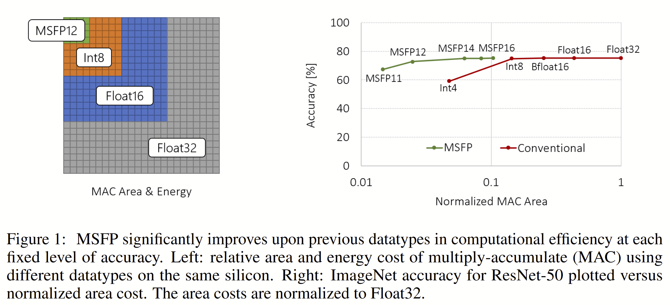
Rouhani et al, Pushing the Limits of Narrow Precision Inferencing at Cloud Scale with Microsoft Floating Point, NeurIPS 2020. DOI. This paper further refines the MS-FP formats from the 2018 paper, and shows “through the co-evolution of hardware design and algorithms, MSFP16 incurs 3× lower cost compared to Bfloat16 and MSFP12 has 4× lower cost compared to INT8 while delivering a comparable or better accuracy.” as illustrated in this figure:
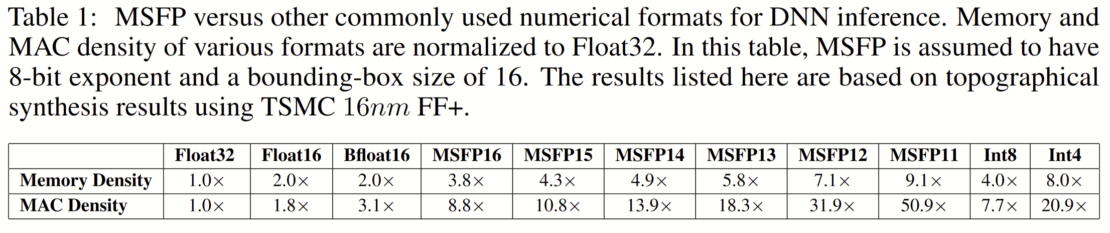
The relative sizes are presented in more detail in this table:
Compelling, right? Compelling enough to justify the extra developer attention, software support, and hardware (quantization and dot products) for these MSFP* formats.
Modern FPGAs with hard block floating point dot product units
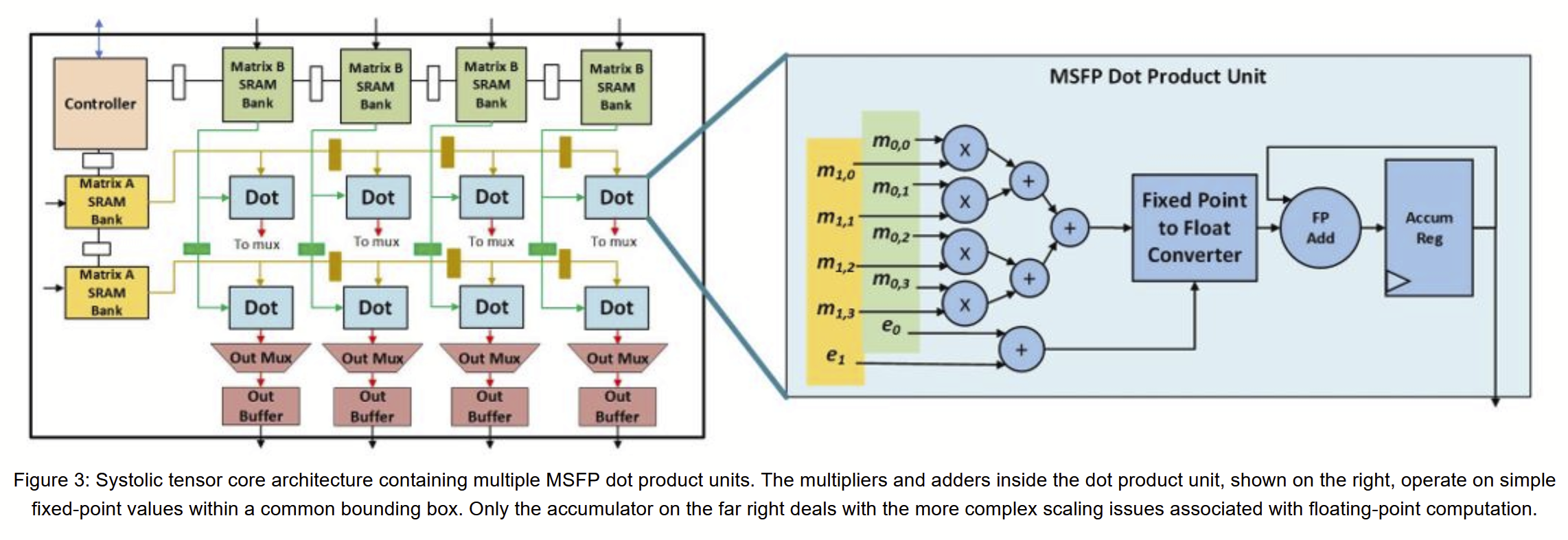
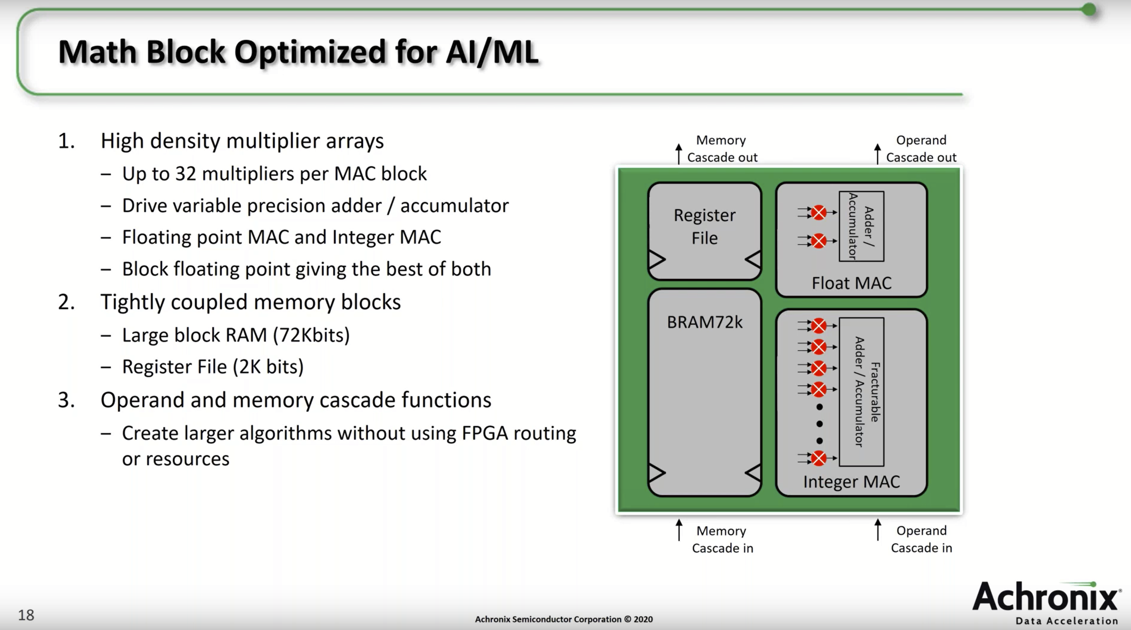
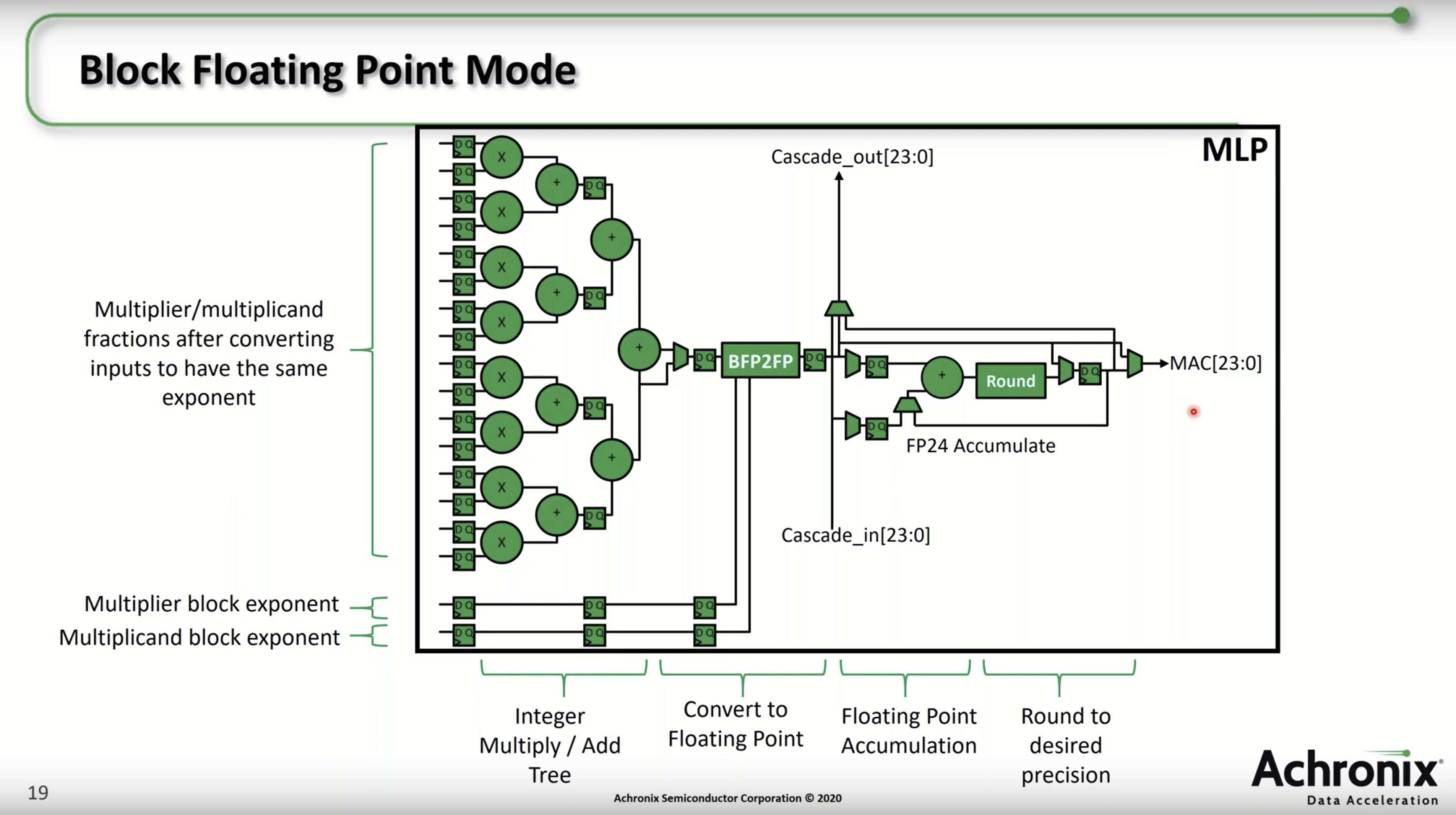
This 2020 Microsoft post also heralds the arrival of hardened BFP dot product units in commercial FPGAs. First introduced in the Achronix Speedster 7t Machine Learning Processor (MLP) blocks in 2019, and then in the Intel Stratix 10 NX (PR)(product brief) in 2020 AI Tensor Block (AITB) units in 2020, these AI tensor math optimized devices provide thousands of hard BFP dot product units. The resemblance to the MSFP Dot Product Unit depicted above is no coincidence. For example, “Working together with our partners in the Intel Programmable Solutions Group (PSG), we’ve delivered significant improvement in area and energy efficiency through silicon hardening”
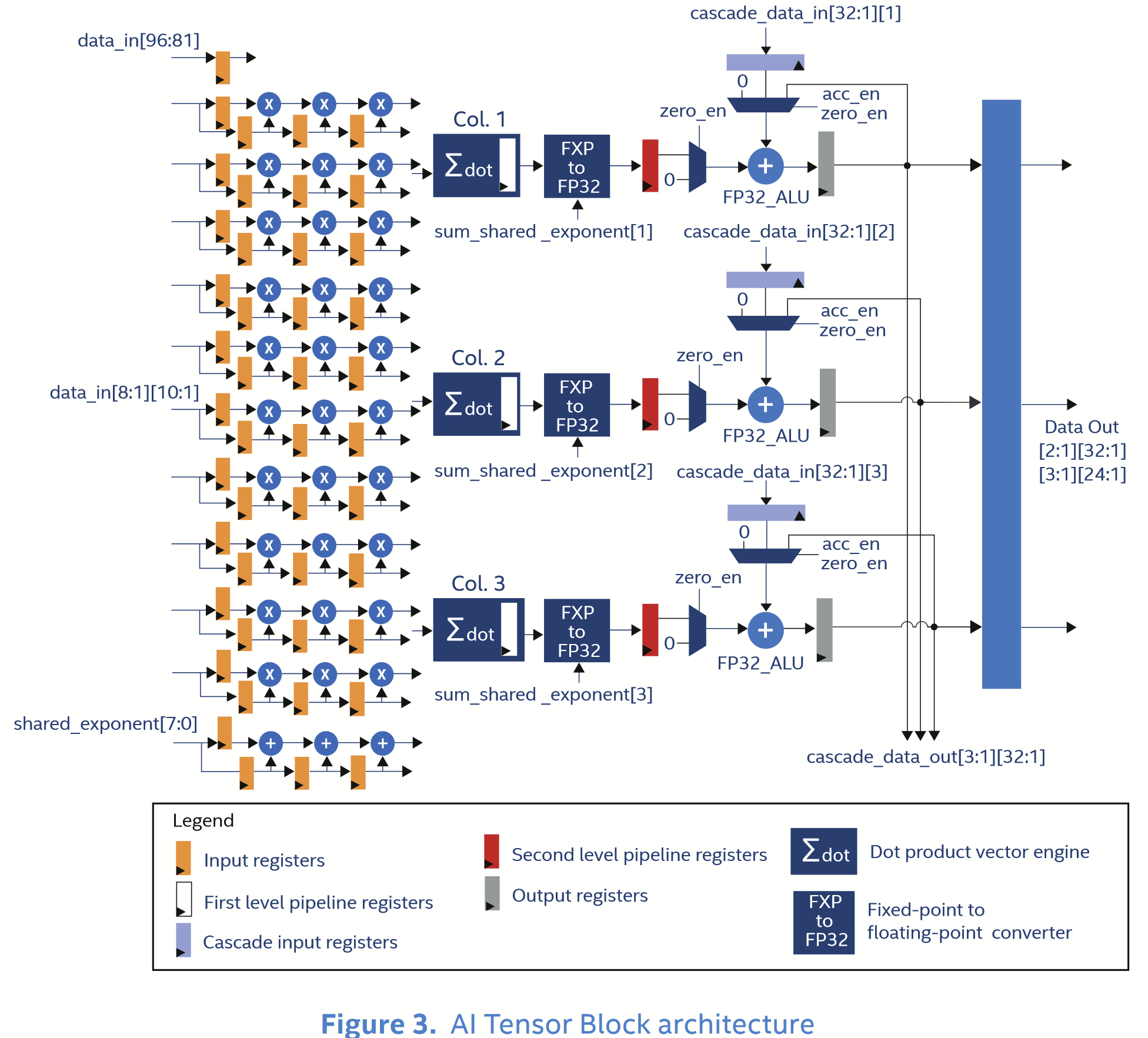
Below is the Intel AI Tensor Block schematic from the white paper. Each block performs up to 30 8b muls, and 30 adds per clock cycle. A Stratix 10 NX has 3960 AITBs so, if you keep it fed and operating at 600 MHz, it performs 3960 × 30 × 2 ops × 0.6 GHz = 143 TOPS — a double that with a 4b mantissa.
Similarly, new Intel Agilex 5 devices have configurable DSP blocks that implement a streamlined tensor block mode with 10 8b muls + product adds per cycle per DSP. (I would have linked to Intel AITB and Agilex 5 tensor block modes’ detailed specs but it seems Intel does not make that available on the web. Dumb.)
In contrast AMD/Xilinx do not presently implement hard block floating point support in their FPGA fabric, instead providing Versal A.I.Engine (AIE) vector processor arrays.
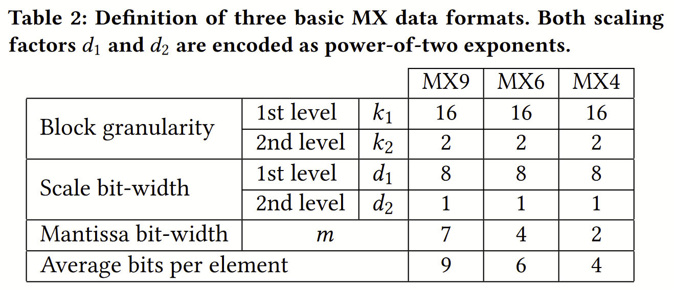
This paper describes a framework Block Data Representations (BDR) to compare the efficiency and quantization loss over a diverse design space of various vector block quantization granularities, with various hierarchies of shared scaling factors, including the 1-level Brainwave block floating point (BFP) formats MSFP*, and novel 2-level shared microexponents (MX) formats, including MX4, MX6, and MX9.
These MX formats are not the MX Alliance formats! Consider Table 2:
If I understand correctly, MX9 is a block of k1=16 elements, all scaled by 2d1, d1 is 8b, further subdivided into 8 subblocks of k2=2 elements, further scaled by 2d2, d2 is 1b, each element being sign × 7b magnitude. In all an MX9 of 16 elements occupies (8b + 8×1b + 16×8b)/16 = 9b per element.
The shared microexponents here contrasts with the present MX Alliance spec, in which each element in an MXINT8, MXFP8 (E5M2 or E4M3), MXFP6 (E3M2 or E2M3), and MXFP4 (E2M1) has a standalone private microexponent (0, 5, 4, 3, 2, 2 bits, respectively).
Or, if you prefer, through the lens of this paper, the MX Alliance MXFP[468] formats are 2-level designs with k1=32 elements, with d1 is 8b, and k2=1 element, with d2 variously 5, 4, 3, 2, 2 bits, respectively.
I wonder what transpired between this ISCA2023 paper and the OCP MX Alliance spec and announcement. I imagine intense multiparty discussions, “can we all please get behind a common MX data schema that evaluates reasonably well on our existing diverse CPUs, GPUs, AIEs, NPUs, etc., that we can evolve future silicon towards, so that we can train our extremely expensive many billion parameter foundational models, just once, and run well on any of them?” If that’s approximately what happened, then any model with k2>1 would probably have been a non-starter. I imagine Microsoft evaluated what became the MX Alliance data formats as part of their BDR parameter sweep and the results were not quite so good as the MX4, MX6, MX9 reported in the ISCA paper, but plenty good enough, in light of this paper, and the MX Alliance white paper: a far superior, drop-in replacement to FP32 and FP16, even for training, and much better QSNR and fewer pitfalls than FP8.
As with the NeurIPS 2020 paper cited above, the evaluations in this paper demonstrate compelling efficiency gains: “MX9 can be used as a drop-in replacement for FP32 or BF16 in the training and inferencing pipeline without the dependency on complex online statistical heuristics or any change in the hyper-parameter settings” and furthermore “MX6 is expected to provide roughly 2× improvement over FP8 in area-memory efficiency and achieves inferences results close to FP32 accuracy with a modest level of quantization-aware fine-tuning.”
The paper also mentions several times the advantages of these MX formats vs. FP8:
“MX9 has a hardware efficiency close to that of FP8 with significantly higher numerical fidelity. For instance, in the case of a Gaussian distribution with variable variance, the QSNR of MX9 is about 16𝑑𝐵 higher than FP8 (E4M3). A 16𝑑𝐵 higher fidelity is roughly equivalent to having 2 more mantissa bits in the scalar floating-point format. For the same distribution, MX6’s QSNR lies between the two FP8 variants E4M3 and E5M2 while providing an approximately 2× advantage on the hardware cost as measured by the normalized area memory efficiency product. We qualitatively observed a similar trend under different data distributions as well.”
Given MX, what FP types are most important in training and inference?
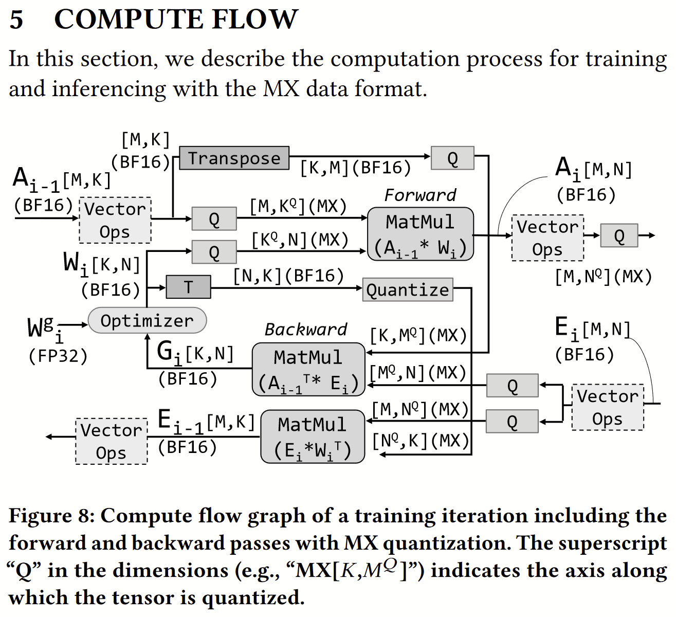
Finally (looking ahead to part two), the paper’s section on Compute Flow is instructive on what kinds of MX data and other reduced precision floating point will be important for ML applications.
Besides myriad MX vector dot products within the MatMuls above, producing BF16 vectors, are quantization operations (along different reduction dimensions) from BF16 to MX, as well as element-wise BF16 vector operations. Is there a need for elementwise MX vector operations, or do MX data live only as fodder for arrays of dot product units within matmuls and convolutions? It seems FP32 and BF16 are necessary: “In our experiments, we use BF16 as the default data format for element-wise operations with the exception of the vector operations in the diffusion loop and the Softmax in the mixture-of-experts gating function.”
It’s also worth noting (section 6.2, Table 4, inferencing) that weights and activations may be kept in different representations (e.g. MX4 weights, MX6 activations) which will merit asymmetric input dot product custom instructions.
Necessity is the mother of invention / “Perspective is worth 90 IQ points”
Wrapping up this part one, some reflection on why it was that Microsoft conceived, refined, perfected, and demonstrated MX format, ahead of all of the other AI focused chip and CSP vendors. Obviously it has much to with Microsoft Research’s decades of work on ML, and then of enterprise and cloud scale ML services, Azure AI services, and Microsoft’s deep expertise operating cloud scale ML workloads, “the world’s computer”, seeing where does the time go and where do the megawatts go.
But for the specific hardware-software codesign insights in MX formats, I think it has a lot to do with their use of FPGAs in Catapult and Brainwave. FPGAs give you a new perspective:
#FPGA Another observation is that although FPGAs are disrespected by elite ASIC designers, the different constraints there afford new insights and spur new approaches that ASIC people may overlook (but ultimately are headed there when the end of Moore’s Law really starts to bite).
#FPGA I used to say you can use today’s FPGAs to build seven year old ASICs — but might also be true that today’s FPGAs help you discover complexity effective design trade offs that will bite ASICs in years to come.
#FPGA Of course things are different in the two worlds — muxes are awful in FPGAs, etc. — but I appreciate the different perspective FPGA implementation affords. “Point of view is worth 80 IQ points” — Alan Kay “I don’t know who discovered water but it wasn’t a fish.”
Gate by gate, wire by wire, FPGAs are often so area and energy inefficient, relative to ASICs, that you just have to find a new, better approach. Those insights can make your FPGA competitive with contemporary ASICs, and give you a leg up when you respin your FPGA design insights into an ASIC of your own. Which Microsoft just did:
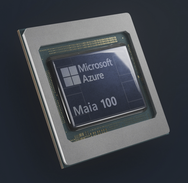
“At Ignite, we’re introducing our first custom AI accelerator series, Azure Maia, designed to run cloud-based training and inferencing for AI workloads such as OpenAI models, Bing, GitHub Copilot, and ChatGPT. Maia 100 is the first generation in the series, with 105 billion transistors, making it one of the largest chips on 5nm process technology. The innovations for Maia 100 span across the silicon, software, network, racks, and cooling capabilities. This equips the Azure AI infrastructure with end-to-end systems optimization tailored to meet the needs of groundbreaking AI such as GPT.”
It’s a lovely thing. Looks like TSMC CoWoS with 4 HBM3 (?) stacks.
“Maia supports our first implementation of the sub 8-bit data types, MX data types, in order to co-design hardware and software,” says Borkar.
In summary
It is a very rare and very special accomplishment for computer architects to define new datatypes that win broad (and TBD: enduring?) industry adoption. Then to go on to design and ship a 100 billion transistor SoC realization of your inventions, a monster with integrated networking and HBM, and advanced packaging, and datacenter scale systems integration! Just stunning. Along the way they also developed Brainwave, the greatest FPGA accelerator that there ever was, and probably that there ever will be. Surely a career highlight for everyone involved. I’m sorry I missed out on all the fun.
Congratulations to Eric Chung, Bita Rouhani, everyone on Catapult, Brainwave, and Maia, and to Microsoft and their partners, on this hardware/software co-design tour de force, the 13+ year harvest of an audacious MSR research agenda and teams built up and tenaciously championed by Doug Burger.
Next time, we’ll explore different approaches to adding MX data type support to RISC-V processors via RISC-V Composable Custom Extensions.
![Excerpt of %5.1 of the spec, illustrating an MX format block with one shared scale X and k scalar elements P[].](https://fpga.org/wp-content/uploads/2023/10/image.png)